Analysis of Multi-Component Dye Baths Using CIELAB, Reflectance Spectrophotometry

Using multi‐component dye baths in anodization processing can be a frustrating endeavor when not equipped with a basic understanding of color theory and how different dyes are affected by various factors.

Jacqueline CookThese factors include but are not limited to disproportionate consumption, vulnerability towards contaminants, and decreased activity over time. By utilizing reflectance spectrophotometry, the data can be quantified and more easily digestible.

Color spaces such as CIELAB and L*C*h, which are used widely by various industries for identifying target shades, can also be used for identifying deviations from a standard.

Introduction

Specialty matches and custom dye mixes have become a less desirable option because of an inability to easily control these baths over time.

As a result, anodizers have lost business with designers. Multi-component organic dyes are difficult to maintain because of a variety of factors, namely disproportionate consumption, and vulnerability towards contaminants, as well as decreased activity over time. As a result, mixes of dyes with three or more components are generally discouraged.

Our original objective was to make these bath adjustments based on transmission results, but it quickly became apparent that this was unlikely to yield practical results as the transmission results were not always correlating with the dyes or the performance of the bath. Reflectance values give us a more accurate and detailed reading of the deviations from the standards that the human eye cannot detect.

In this paper, we intend to provide a control method to offer better color consistency and better control of custom color mixes using reflectance spectrophotometry and L*a*b* data.

Color Theory

In order to better interpret our findings, a review of color theory is in order. Color is the human eye’s perception of reflected radiation in the visible region of the electromagnetic spectrum (400–700 nm).

There are three descriptive terms used to characterize color:

Lightness - How bright or dark a color is.
Hue - Where a color falls on the color wheel.
Saturation - How vivid or dull a color is.

The terms are visualized in Fig. 1. The color wheel [Fig. 1(a)] shows how these colors interact. Colors on the opposite sides of the wheel will cancel out, while colors 30 degrees clockwise or counterclockwise will merely shift the hue one way or another (e.g., adding green to red vs. adding yellow or blue). Figures 1(b and c) show the interactions between lightness and saturation. Moving vertically changes the lightness, while moving horizontally changes the vividness.

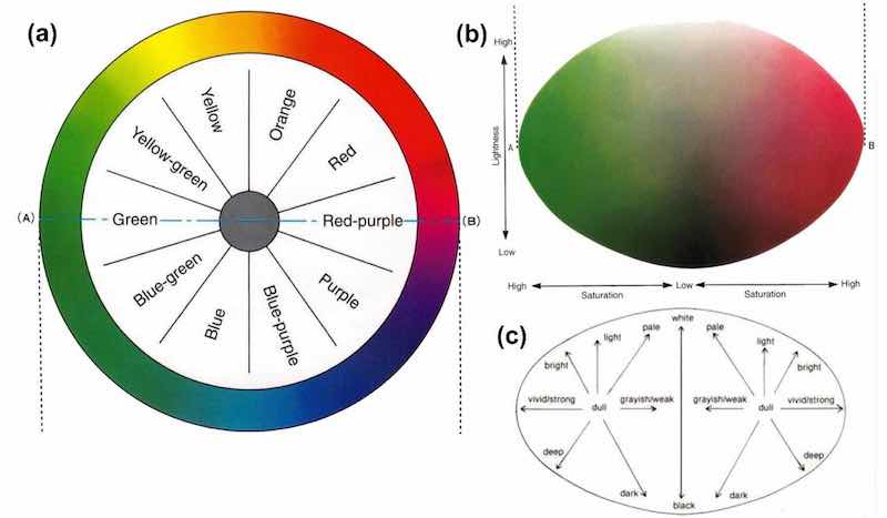Figure 1 – Characterization of color properties: (a) color wheel; (b) changes in lightness and saturation for red-purple and green; (c) adjectives related to colors for lightness and saturation.

Having defined ways to describe color, we can measure them and assign numerical values. This has created several different color spaces, which are defined as methods for expressing the color of an object or a light source using some kind of notation, such as numbers. The most commonly used color spaces are the L*a*b* and L*C*h* systems.

**Lab* Color Space**

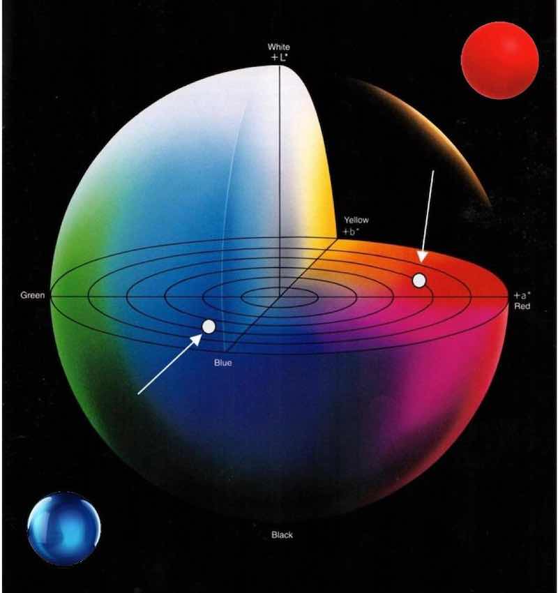Figure 2 – L*a*b* color space.L*a*b* color space (Fig. 2) is also referred to as the CIELAB system and is considered the better-known of the two. It can be visualized as a spherical coordinate system in which the vertical axis is the lightness variable L*, ranging from 0% (black) to 100% (white), and the radii in the horizontal plane are the chromaticity variables a* and b*.

Variable a* is the green (negative) to the red (positive) x-axis, and variable b* is the blue (negative) to the yellow (positive) y-axis. The center is achromatic, meaning there is no saturation of color, leaving a grayish hue.

Defining the red ball in the upper right corner of Fig. 2 in L*a*b* color space would be L* = 43.31, a* = 47.63, and b* = 14.12. Similarly, the blue ball in the lower left would be measured as L* = 57.40, a* =-15.64, and b* = -40.33.

**Lch* Color Space**

In L*c*h* color space (Fig. 3), L* indicates lightness, C* represents chroma, and h is the hue angle.

Fig. 3 L*c*h* color space.The value of chroma C* is the distance from the lightness axis (L*) and starts at 0 in the center. The hue angle starts at the +a* axis and is expressed in degrees (e.g., 0° is +a*, or red, and 90° is +b, or yellow). As a result, the L*C*h* values of a color will always be positive.

With the same red dot from Fig. 2, the L*C*h* measurement would be L* = 43.31, C* = 49.68 and h* = 16.50.

Color Measurement

Let us consider the two primary methods of color measurement: transmission spectroscopy and spectral reflectance. Transmission spectroscopy [Fig. 4(a)] involves projecting a light source through a sample. The method of analysis is based on the absorption of the infrared beam by a sample at specific wavelengths or frequencies of light. Spectral reflectance [Fig. 4(b)] is a measure of how much energy (as a percentage) a surface reflects at a specific wavelength. Many surfaces reflect different amounts of energy in different portions of the spectrum.

Our original intention was to analyze our sample dye baths using transmission, providing a more simple and efficient way to adjust dye baths. However, it became immediately clear that this would not be the most effective method for analyzing dyes baths as the change in color of the bath and its parts were not the same. Nonetheless, using spectrophotometers and colorimeters provides greater insight into how to color changes far more so than the naked human eye.

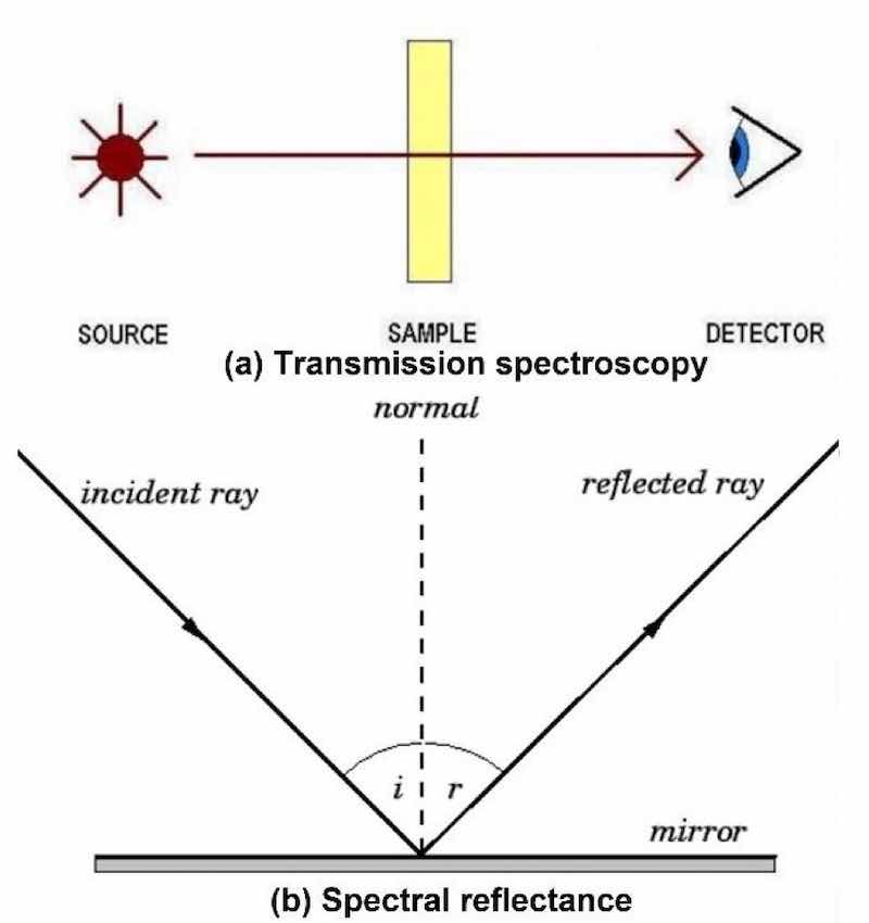Figure 4 – Color measurement methods

Reflectance data (Fig. 5) can be obtained using a spectrophotometer, standardized with a pure white standard (100% reflectance) and a black box (0% reflectance). These will show up as relatively straight lines at or near 0 and 100 percent. These readings produce spectral reflectance graphs in which the x-axis is the wavelength (nm), and the y-axis is percent reflectance. These are shown in the figure for primary blue, green, and red, as well as a grey scan.

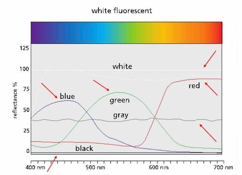Figure 5 – Spectral reflectance plots for primary colors and grey, showing white and black lines for standardization.

Case Study #1: Green AEN

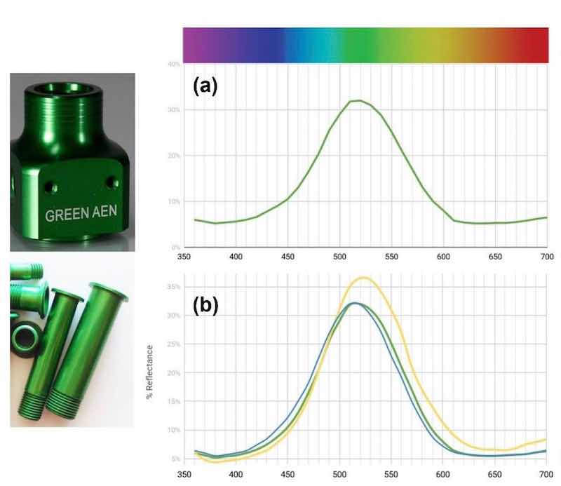Figure 6 – Reflectance curves for two-component Green AEN dye: (a) standard make-up; (b) effect of separately increasing blue and yellow components.Green AEN is a popular two-component dye with a tendency to shift over time. As seen on the reflectance graph [(Fig. 6a)], there is a spike at 520 nm, which, as we know, represents the green. Meanwhile, there are transitions between yellow and blue, the two dyes needed to make this color.

Reflectance data was taken from two parts - one with 10% more yellow and one with 10% more blue - to show how the reflectance graph shifts [(Fig. 6(b)]. As shown, the blue curve shows a shift to the left. The yellow curve has a higher reflectance from 490 nm on because yellow appears lighter.

In the following discussion(s), it should be noted that the tabular data refers to the change in the L*a*b* and L*C*h* numbers from those derived from the standardized make-up, i.e., DL, Da, Db, DC, and DH, with DL applying to both L*a*b* and L*C*h* number sets. DE represents the overall change and is an amalgamation of the L*a*b* numbers. D can be considered a delta (Δ) value.

For the first part of this experiment, we ran parts continuously through a small bath (50 mL) until approximately 150 in2 had been processed and significant changes could be seen. As can be seen in the graph of Fig. 7, the reflectance is significantly higher across the board, indicating that the part is lighter overall. Note that DL shows the largest change, signifying that the “exhausted bath” sample is lighter. A 27% add of Green AEN was made to return the dye back to its original strength.

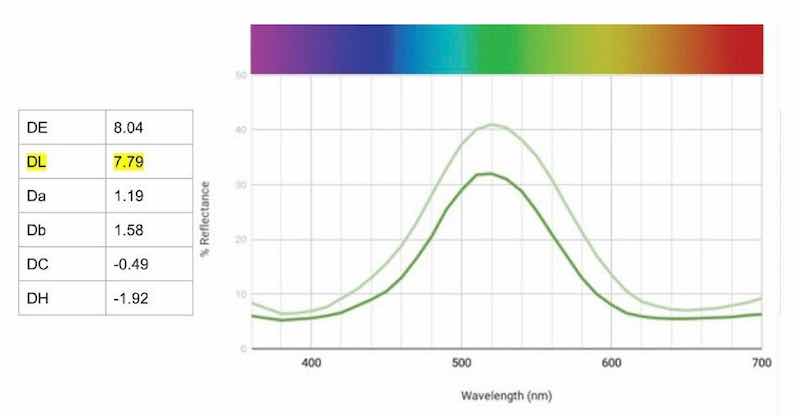Figure 7 – Change in reflectance curves with “exhausted” Green AEN bath. strength.While analyzing the reflectance charts, note the changes at the peaks and the transition areas of known dye components. For example, the largest percentage change of 9% can be found at the peak of 510 nm, supporting the data DL that the bath is lighter.

To determine the effects of contaminants in the process, 1000 ppm of sulfate was added to a fresh bath. As seen on the reflectance graph of Fig. 8, the sulfate contamination had a greater effect on the yellow in the dye. Accordingly, about 4% of the yellow was added, as well as 15% of the green, to increase the strength.

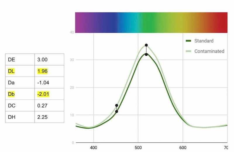Figure 8 - Change in reflectance curves with Green AEN bath with 1000 ppm sulfate contamination.Wrapping up our work with Green AEN, we analyzed a random customer bath compared to a standard. While the sample’s reflectance data generally follows the standard curve [Fig. 9(a)], we can see that it shifts more yellow and is weaker. We started by making an adjustment to the hue with a 10% add of the blue, then an 8% add of Green AEN [Fig. (9b)]. The results are a graph that basically follows the standard curve and has a significantly lower DE. It is important to realize that some dyes cannot return to the exact standard as they lose saturation of color over time. This can be seen in the Da value of the adjusted bath. It is simply not as green as the standard.

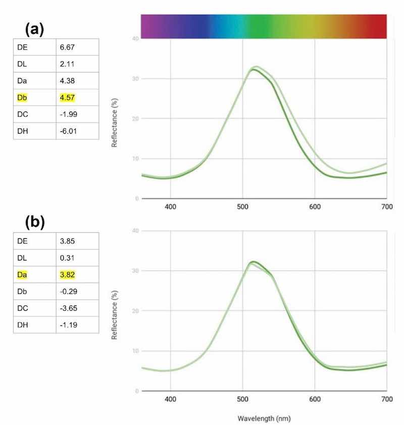Figure 9 - Change in reflectance curves with Green AEN customer bath requiring analysis and adjustment.

Case Study #2: Coyote Brown

Figure 10 – Range of shades in Coyote Brown specification.Coyote brown is a popular request for shade matches, mainly used for military specifications. For this specific match, we recommended a combination of 40% Bronze 2LW (a reddish bronze) and 60% Grey HLN (a greenish grey). This specification is not extremely precise. The parts shown in Fig. 10 show that the color can range from more red, like (a) the knife, or more green, like (b) the gun. The match that we selected looks most like (c) the clip in the center, allowing room for change shifting in either direction.

Colors with less saturation, such as greys and browns, tend to have a flatter curve.

Figure 11 – Reflectance curves for two- component Coyote Brown dye: (a) standard make-up; (b) effect of separately increasing grey and bronze components.As shown in Fig. 11(a), with this dye, small spikes can be seen at 380 nm, 530 nm, and a large spike going gradually up to 700 nm. This indicates that the predominant color in this dye is red. This is also where we see the largest deviations from the standard. As in the Green AEN study, two baths were made up with a 10% strength change in either component to better understand how this would look on a reflectance graph [Fig. 11(b)]. The largest change was observed between 620 to 700 nm, where the bronze made the bath redder and the grey - with its green components - worked to neutralize it. 1000 ppm of sulfate was added to the bath to see if it affected one dye more than the other.

According to the graph in Fig. 12, the change in this dye resulting from contamination was an overall lightening. A significant add of 110% was required to bring the dye back to standard strength. In practice, it would be easier at that point to make up a fresh bath.

Finally, a randomly selected commercial bath was analyzed and compared to the standard bath, shown in Fig. 13(a). While the L* value was virtually unchanged, the a* and b* values were both significantly different, greatly affecting the DE value. This bath was greener and bluer than the standard, implying that there was more grey than bronze in it versus the standard.

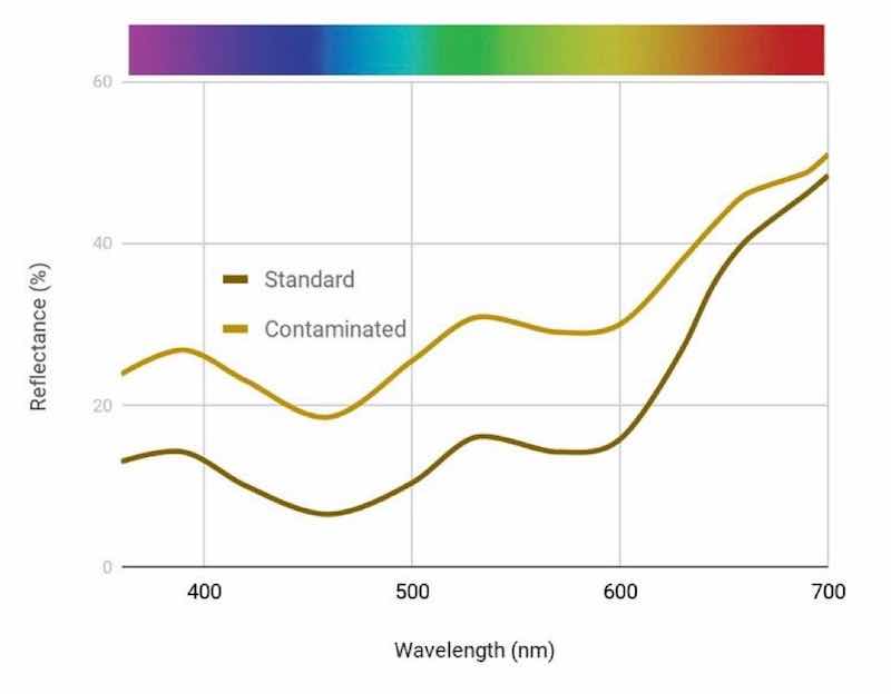Figure 12 - Change in reflectance curves with Coyote Brown bath with 1000 ppm sulfate contamination.In order to rectify this, an add of about 40% Bronze 2LW was added to the bath [Fig. 13(b)] to shift it back to the standard. Doing this in our lab setting, this add also significantly affected the concentration, requiring a dilution of the bath by 20%.

Case Study #3: Black MLW

Black MLW is a three-component dye made mostly with a blue-black and less than 10% of an orange and a reddish brown. Remembering the color wheel [Fig. (1a)], the orange and brown work together to neutralize the blue of the dominant dye. For the purposes of this experiment, we made up the MLW bath at 2 g/L in order to more easily see the changes in color. Similar to the coyote brown, the reflectance graph is mostly flat because of the lack of saturation in the dye (Fig. 14).

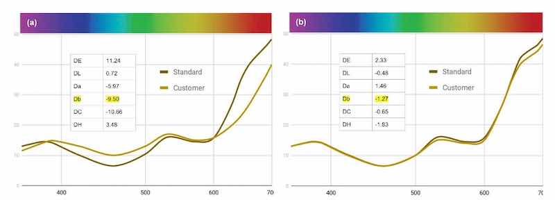Figure 13 - Change in reflectance curves with Coyote Brown customer bath requiring analysis and adjustment.

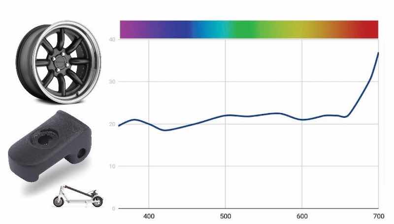Figure 14 – Reflectance curve for standard make-up of three-component Black MLW dye.As with the Green AEN trial, we began our study by exhausting the bath to see how it shifted over time. As noted in Fig. 15(a), the obvious overall lightening and a shift to a bluer hue are evident. On a processing line, this is the point where an add of the dye is needed. In our study, we added about 40% MLW. With this data, we see that the bath is producing parts that are significantly bluer ([Fig. (15(b)]. By adding <0.5% of the brown and orange, we can neutralize the blue and a bit of the green that are flaring. This brought the dye bath back to the standard with a DE of 2.6.

The most detrimental contaminant for Black MLW is aluminum. Accordingly, we added 100 ppm of aluminum to a bath and let it stand overnight to see its response at this high level of contamination, and then see if the bath could be salvaged.

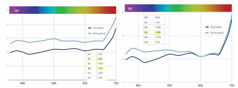Figure 15 - Change in reflectance curves with (a) “exhausted” Black MLW and (b) its restoration with an add of 40% MLW.

Reflectance readings show that the aluminum affected the brown and orange tints more than the blue of the bath, causing a significant shift around 420 nm and 600-630 nm [Fig. 16(a)]. An add of around 1% of the orange and brown combined was added to bring the dye bath back but that caused the bath to shift to yellow. After an addition of the blue-black dye, we returned the dye back to the standard [Fig. 16(b)].

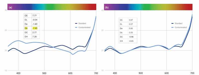Figure 16 - Change in reflectance curves of Black MLW dye with (a) 100 mL aluminum contamination and (b) its restoration with adds of 1% orange and brown components and blue-black as required.

For the last part of this trial, we again tested a customer bath to see if we could return it to standard performance. We started by diluting the bath to 2 g/L, and obtained the results shown in Fig. 17(a). After an add of 1% of the orange and 1% of the brown as well as a dilution of 10%, we restored dye back to the benchmark standard [Fig. 17(b)].

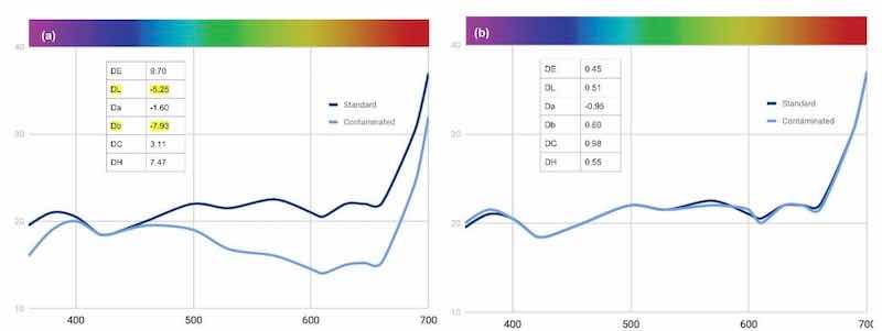Figure 17 - Change in reflectance curves with Black MLW customer bath requiring analysis and adjustment.

Summary

This paper has reviewed color theory, color spaces, and how to use quantified data in order to manage multi‐component dye baths using reflectance spectrophotometry. This technique is effective in determining the condition of dye baths for anodized products, monitoring the bath condition and chemistry, and troubleshooting the process online.

Armed with a better understanding of how to analyze quantified data, we can more effectively and efficiently make the necessary changes to an ever evolving bath to increase longevity and consistency on our line.

References

Jacqueline Cook is a Technical Representative at Reliant Aluminum Products, LLC, in High Point, North Carolina. Visit https://reliantaluminumproducts.com. Compiled by Dr. James H. Lindsay, Technical Editor - NASF